准备工作 🔗
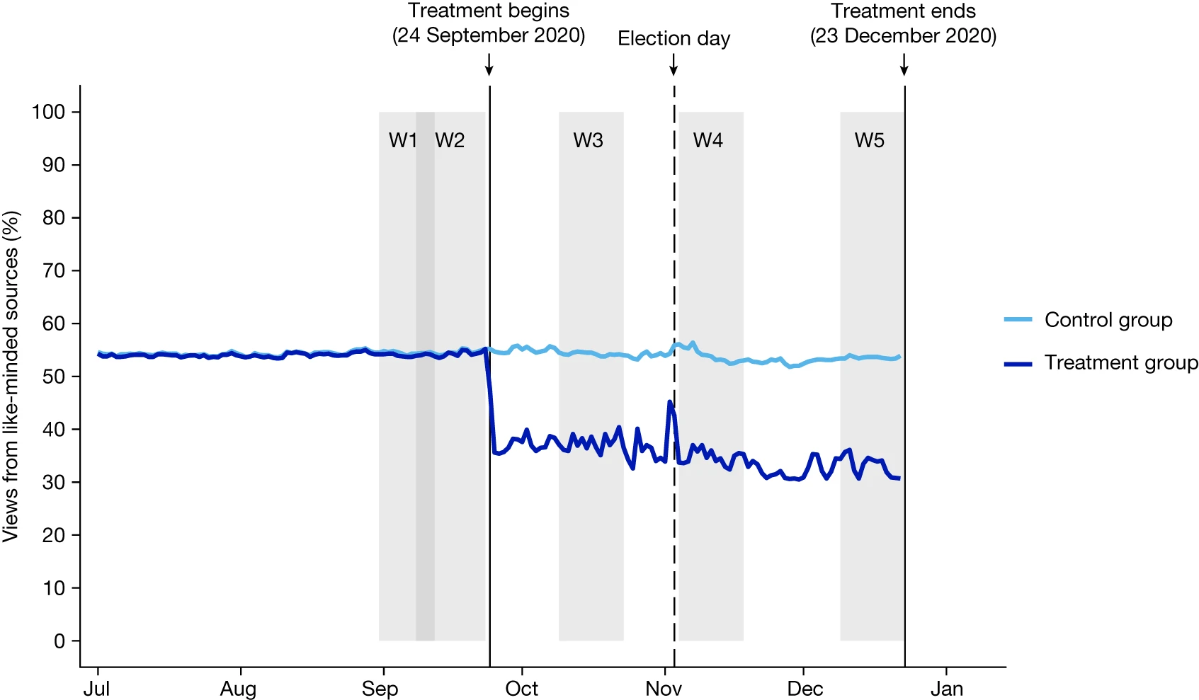
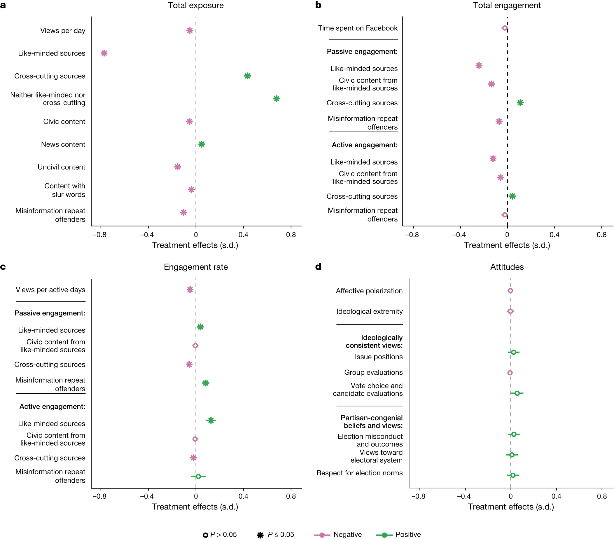
复现七月发表在nature的Like-minded sources on Facebook are prevalent but not polarizing里的figure2 和figure3。原图如下:
文献提供了原始数据集,下载到本地直接使用。set up R, 加载需要用到的R包:
xfun::session_info()
library(readr) ## 读取数据
library(ggplot2) ## 画图
library(dplyr) ## pipe
Figure 2 🔗
先看看数据,有三个变量,分别对应X,Y和分组。并且观察到所有的变量类型全部是我们希望的变量类型,可以直接画图啦👏
fb_figure2 <- read_csv("https://lin-yu.me/posts/2023_08_10fb/data/2023_08_10fb/fb_figure2.csv")
fb_figure2 %>% tibble()
先画大体的框架:
- ggplot aes: color = treatment_group;
- geom_line: 线图,按照treatment_group变量分类;
- geom_vline: 画垂直线,其中一条linetype=dashed;
- annotate: 增加‘text’,‘rect’两种注释
fb_figure2_out <- fb_figure2 %>%
  ### 框架 ###
  ggplot(aes(x = vpv_date, y = like_minded, color = treatment_group)) +
  geom_line(size=1.2,alpha=2) +
  ### 加3条垂直线 ###
  geom_vline(xintercept = as.Date("2020-09-24")) +
  geom_vline(xintercept = as.Date("2020-11-03"), linetype = "dashed") +
  geom_vline(xintercept = as.Date("2020-12-23"))+
  ### 加框选框以及文字 ### 一个annotate框对应一个annotate文字,形成一组
  annotate("rect",
           xmin = as.Date("2020-09-01"),
           xmax = as.Date("2020-09-15"),
           ymin = 0,
           ymax = 0.9,
           alpha = 0.2
  ) +
  annotate('text',
           label = 'W1',
           x = as.Date("2020-09-05"),
           y = 0.89
  )+
  annotate("rect",
           xmin = as.Date("2020-09-08"),
           xmax = as.Date("2020-09-23"),
           ymin = 0,
           ymax = 0.9,
           alpha = 0.2
  ) +
  annotate('text',
           label = 'W2',
           x = as.Date("2020-09-18"),
           y = 0.89
  )+
  annotate("rect",
           xmin = as.Date("2020-10-08"),
           xmax = as.Date("2020-10-20"),
           ymin = 0,
           ymax = 0.9,
           alpha = 0.2
  ) +
  annotate('text',
           label = 'W3',
           x = as.Date("2020-10-14"),
           y = 0.89
  )+
  annotate("rect",
           xmin = as.Date("2020-11-03"),
           xmax = as.Date("2020-11-15"),
           ymin = 0,
           ymax = 0.9,
           alpha = 0.2
  ) +
  annotate('text',
           label = 'W4',
           x = as.Date("2020-11-08"),
           y = 0.89
  )+
  annotate("rect",
           xmin = as.Date("2020-12-12"),
           xmax = as.Date("2020-12-23"),
           ymin = 0,
           ymax = 0.9,
           alpha = 0.2
  )+
  annotate('text',
           label = 'W5',
           x = as.Date("2020-12-18"),
           y = 0.89
  )+
  ### 加上段的标注文字 ###
  annotate("text",
           label = "Treatment begins \n (20 September 2020) \n ↓",
           x = as.Date("2020-09-24"),
           y = 1
  ) +
  annotate("text",
           label = "Election day \n ↓",
           x = as.Date("2020-11-03"),
           y = 1
  ) +
  annotate("text",
           label = "Treatment ends \n (23 December 2020) \n ↓",
           x = as.Date("2020-12-23"),
           y = 1
  )
输出如下图像:
看上去还不错,整体还是像模像样的!这里可以看到两个问题:
- 三条垂直线有点长,挡住了最上面的注释;
- 最后一个注释因为X轴取值范围的原因被挡住了,未显示完全;
解决方案如下:
- 我们用geom_segment取代geom_vline
- 通过scale_x_date对X轴的范围进行自定义,使end date更长一些
此外,我们还需要对图形进行精修,包括:
- scale_x_date/ 自定义X轴,x-axis名字
- scale_y_continuous 自定义Y轴的format(这里是percent),range和title
- scale_color_manual 自定义color,legend title, 分组label
- theme里面定义grid为无,并且background为白色,x-axis 和y-axis为实线
原始画垂直线代码:
geom_vline(xintercept = as.Date("2020-09-24")) +
  geom_vline(xintercept = as.Date("2020-11-03"), linetype = "dashed") +
  geom_vline(xintercept = as.Date("2020-12-23"))
替换代码:
 geom_segment(
  aes(
    x = as.Date("2020-09-24"),
    y = 0,
    xend = as.Date("2020-09-24"),
    yend = 0.93
  ),
  color = "black"
) +
  geom_segment(
    aes(
      x = as.Date("2020-11-03"),
      y = 0,
      xend = as.Date("2020-11-03"),
      yend = 0.93
    ),
    color = "black",
    linetype = "dashed"
  ) +

  geom_segment(
    aes(
      x = as.Date("2020-12-23"),
      y = 0,
      xend = as.Date("2020-12-23"),
      yend = 0.93
    ),
    color = "black"
  )
通过scale_x/y/color等精修:
- 这里的日期我们的format用的是%b 其他的format cheat sheet 可以在这里找到
- 因为系统语言是中文,format也会是中文的日期,如果想要改为英文的日期format,可以在画图之前运行Sys.setlocale(“LC_ALL”,“English”)设置为英文。(用Sys.getlocale()判断当前语言系统)
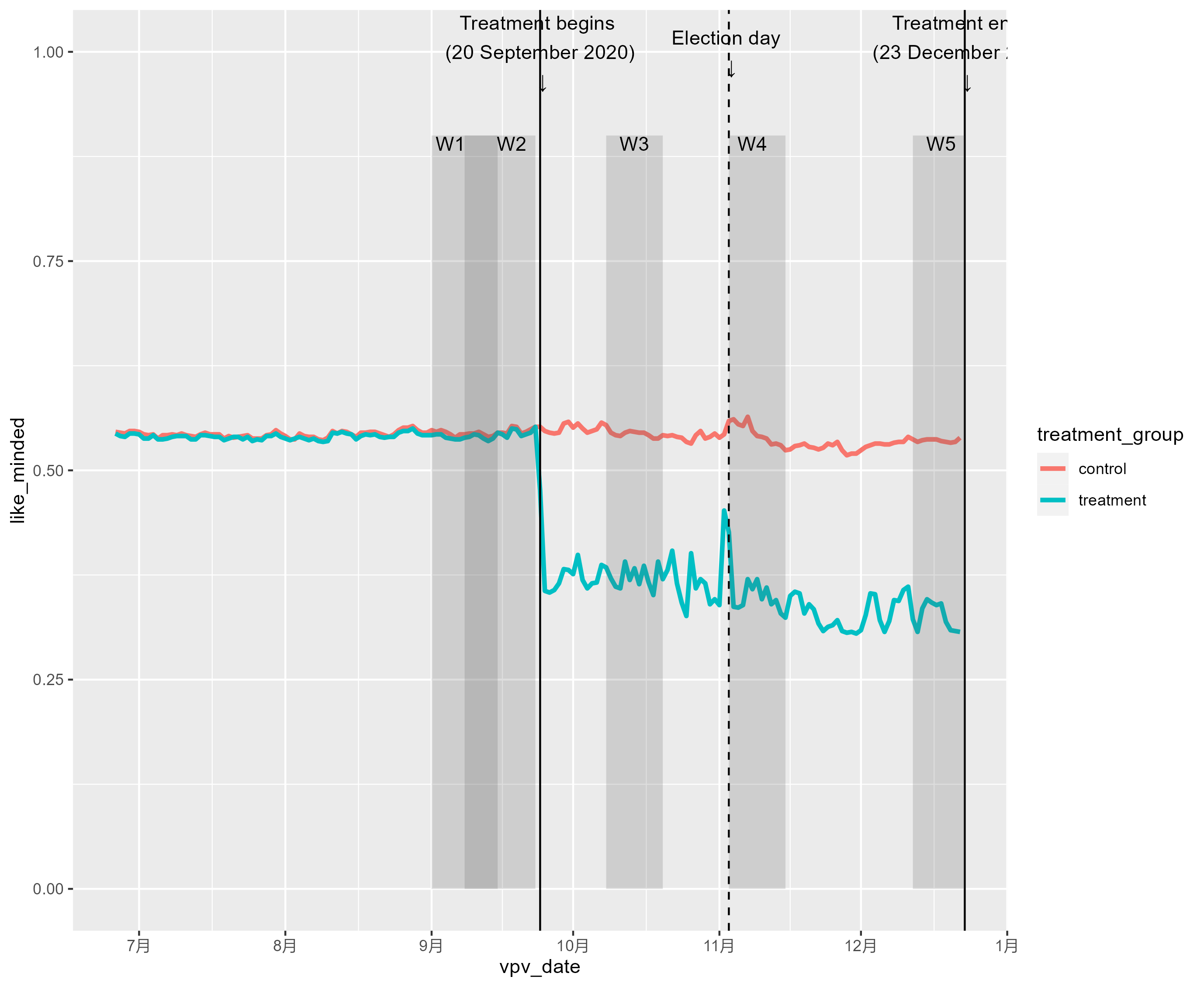
fb_figure2_out +
  scale_y_continuous(
    name = "Views from like-minded sources",
    labels = scales::percent,
    limits = c(0, 1), ## range
    breaks = seq(0, 1, 0.1) ## 定义ticks
  ) +
  scale_x_date(
    name = "",
    date_breaks = "1 month",
    date_labels = "%b",
    limits = c(as.Date("2020-06-15"), as.Date("2021-01-01"))
  ) +
  scale_color_manual(
    name = "",
    values = c("#2b8cbe", "#0055FF"),
    labels = c("Control group", "Treatment group")
  )+
theme(
  panel.grid = element_blank(),
  panel.background = element_rect(fill = "white"),
  axis.line = element_line(color = "black")
)
完美复现:
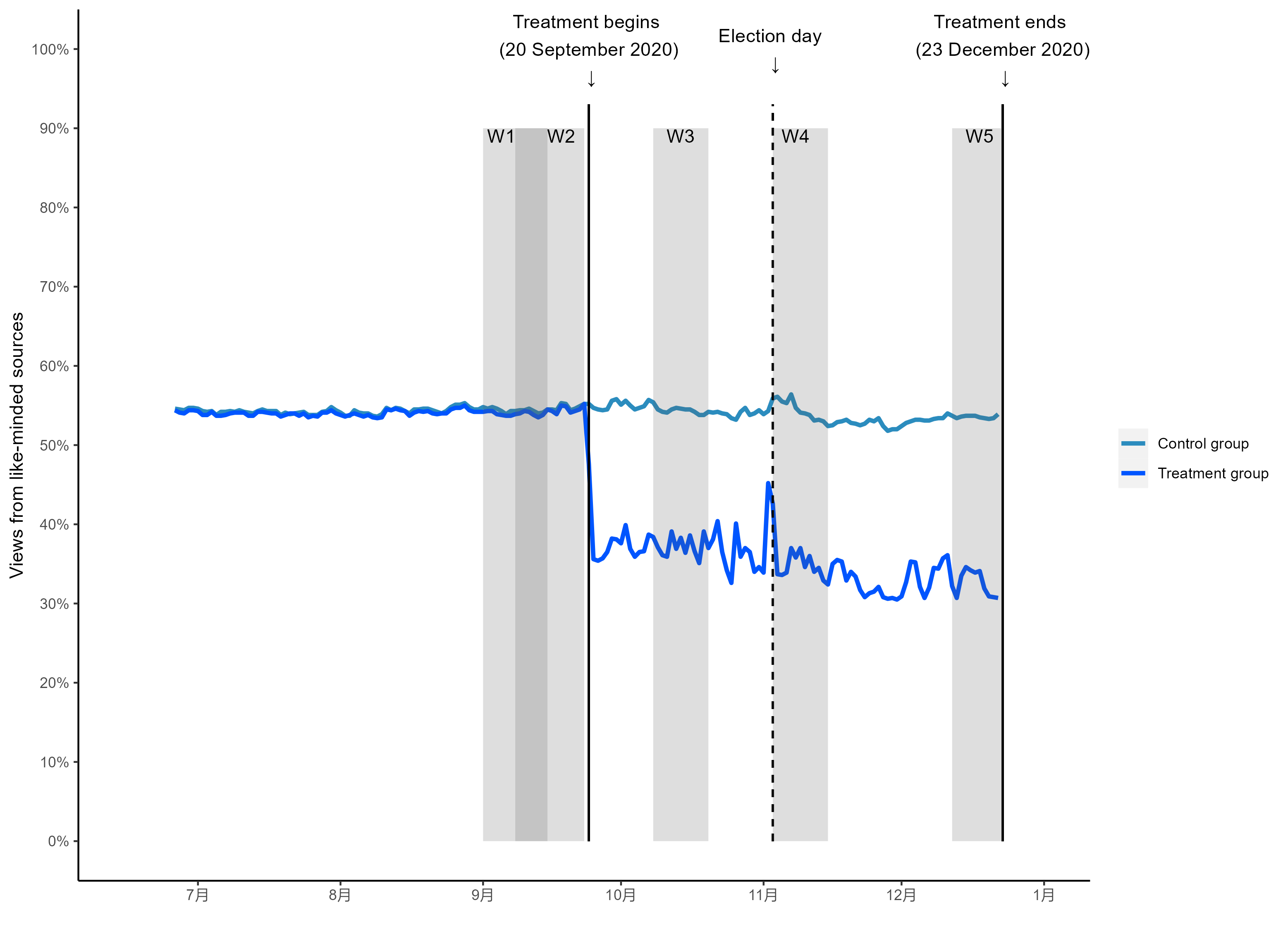
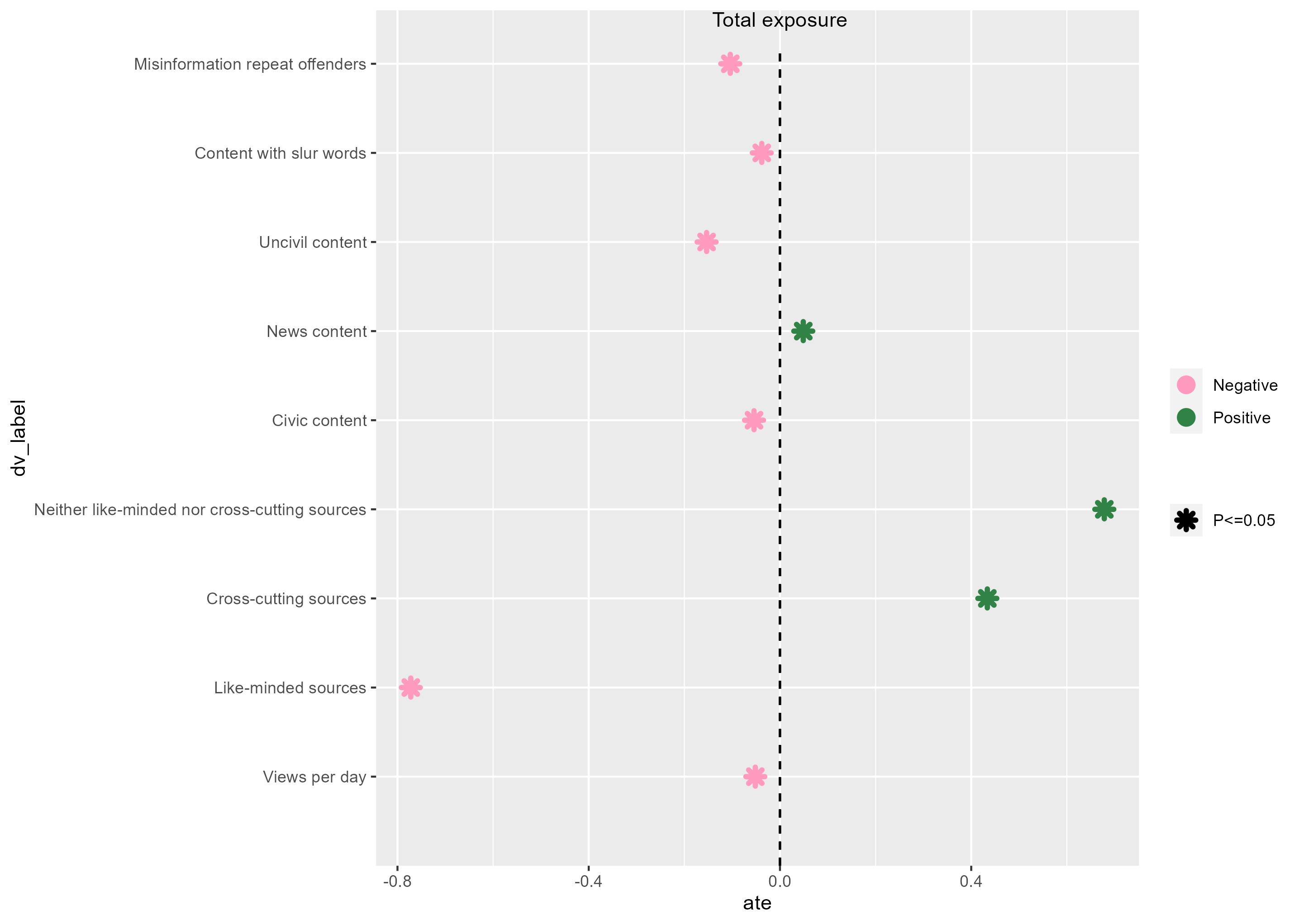
Figure 3 🔗
由于ABCD四张图类似,这里只复现AB两图。
A图 🔗
fb_figure3 <- read_csv("https://lin-yu.me/posts/2023_08_10fb/data/2023_08_10fb/fb_figure3.csv")
先准备A图的数据: 原数据集是把ABCD四个图的数据放在一个dataset里的,所以我们可以:
- 先把A图数据filter出来,并且将我们的Y轴字段转化为一个factor类型的变量,以便输出的Y轴顺序是我们desired顺序。
- 因为原图有按照ate取值的正负和significance来分组,所以生成这两个新变量
fb_figure3_a <- fb_figure3 %>%
  filter(str_detect(facet_label, "A\\)")) %>%
  mutate(
    neg_pos = ifelse(ate < 0, "Negative", "Positive"),
    sig = ifelse(pval <= 0.05, "P<=0.05", "P>0.05")
  ) %>%
  mutate(dv_label = factor(dv_label,
    levels = c(
      "Views per day",
      "Like-minded sources",
      "Cross-cutting sources",
      "Neither like-minded nor cross-cutting sources",
      "Civic content",
      "News content",
      "Uncivil content",
      "Content with slur words",
      "Misinformation repeat offenders"
    )
  )) %>%
  arrange(desc(dv_label))
同样地,我们先搭框架:(用stroke可以控制散点加粗)
 fb_figure3_a %>%
  ggplot(aes(x = ate, y = dv_label)) +
  geom_point(aes(color = neg_pos,
                 shape = sig),
             size = 2,
             stroke = 2)
然后加入annotation (geom 貌似可以用richtext选项,虽然我没有成功,好在我的label不需要加CSS,无妨)
geom_segment(
    aes(
      x = 0,
      xend = 0,
      y = 0,
      yend = 9.2
    ),
    color = "black",
    linetype = "dashed"
  ) +
  annotate(
    geom = "text",
    x = 0,
    y = 9.5,
    label = "Total exposure"
  )
接着我们来定义散点的颜色和形状:
  scale_color_manual(
    name = "",
    values = c("#FF99BF", "#308344")
  ) +
  scale_shape_manual(
    name = "",
    values = c(8, 1)
  )
至此得到的图形也是八九不离十了,这里的takeaway是,对于离散的Y变量,在geom_segment里面居然还是可以用坐标来表示!图形长这个样子:
我们还解决的问题是:
- scale_x_continuous 来控制X轴的range,breaks;scale_y_discrete的limits来控制各个factor的顺序(因为我发现,即使在最开始准备数据集时,已经定义了levels,但散点图的Y轴顺序仍然不是desired order。)
- theme的设置:panel.background, x/y line, ticks
  scale_y_discrete(
    name = "",
    limits = rev(levels(fb_figure3_a$dv_label))
  )+
  scale_x_continuous(
    name = "Treatment  effects (s.d.)",
    limits = c(-0.8, 0.8),
    breaks = seq(-0.8, 0.8, 0.4)
  ) +
  # theme(axis.text.x = element_text(angle = 90))+
  theme(
    panel.background = element_rect(fill = "white"),
    axis.line = element_line(color = "black"),
    axis.ticks = element_blank(),
    legend.position = "bottom"
  )
嗯挺不错,A图完成:
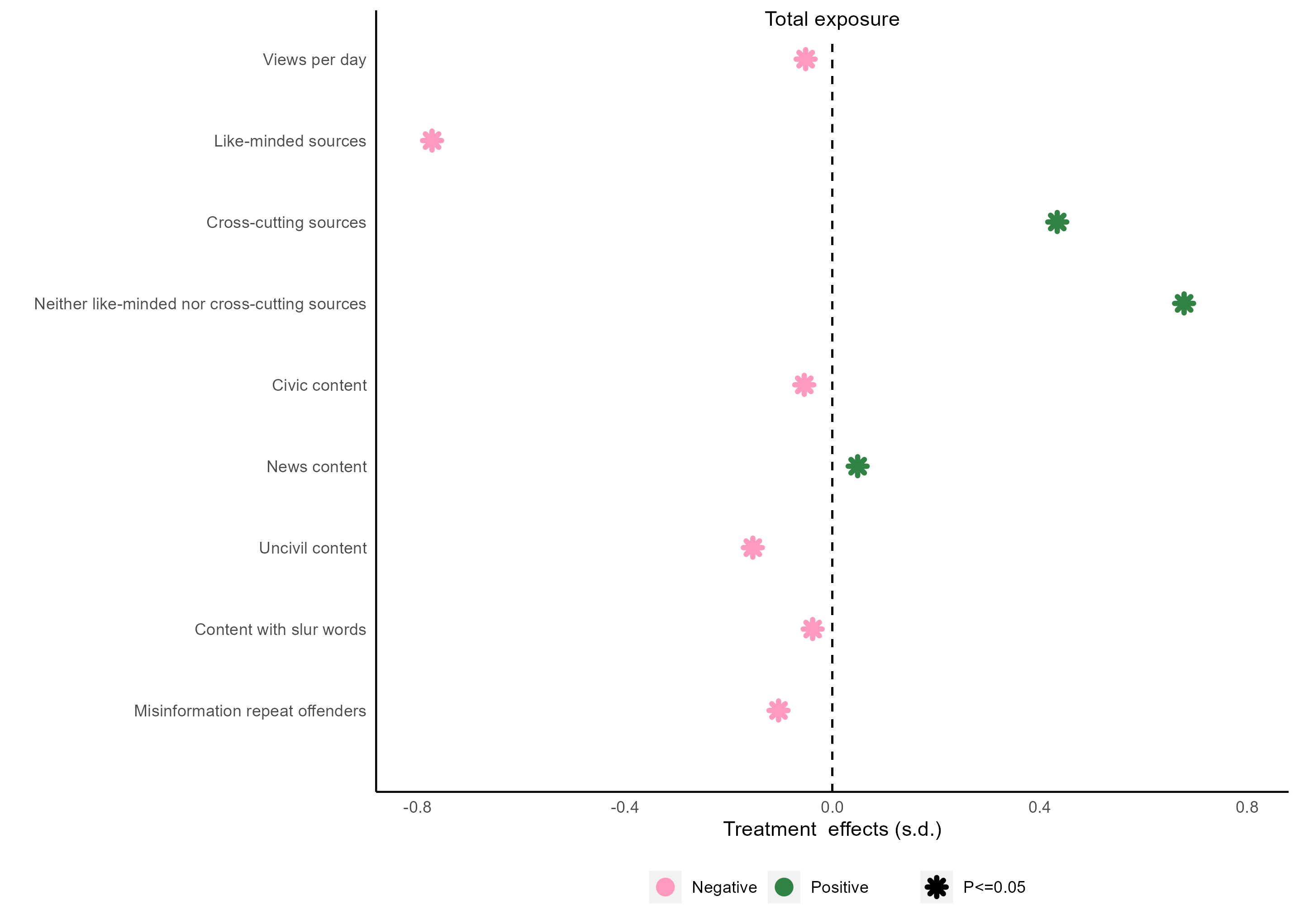
B图 🔗
先准备数据集,这里我们观察一下可以发现,除了要对B图数据进行A图类似的准备之外,B图中的Y被分为了3个类别:
- Time spent on Facebook
- Passive engagement
- Active engegement
并且我们的大类标签还是被加粗的!
所以我们可以:
- 给数据集合增加两行新数据,只有Y轴,但没有其他取值;
- 生成一个face变量,控制Y轴各个值face value是plain还是bold.
fb_figure3_b <- fb_figure3 %>%
  filter(str_detect(facet_label, "B\\)")) %>%
  mutate(
    neg_pos = ifelse(ate < 0, "Negative", "Positive"),
    sig = ifelse(pval <= 0.05, "P<=0.05", "P>0.05")
  ) %>%
  bind_rows(data.frame(dv_label = c(
    "--------------------------------\n Passvie engagement:",
    "--------------------------------\nActive engagement:"
  ))) %>%
  mutate(dv_label = factor(dv_label,
    levels = c(
      "Time spent on Facebook",
      "--------------------------------\n Passvie engagement:",
      "Passive eng. w/like-minded sources",
      "Passive eng. w/civic content\nfrom like-minded sources", "Passive eng. w/cross-cutting sources",
      "Passive eng. w/misinformation repeat offenders",
      "--------------------------------\nActive engagement:", "Active eng. w/like-minded sources",
      "Active eng. w/civic content\nfrom like-minded sources", "Active eng. w/cross-cutting sources",
      "Active eng. w/misinformation repeat offenders"
    )
  )) %>%
  mutate(face = ifelse(is.na(ate), "bold", "plain")) %>%
  arrange(desc(dv_label))
接着也是进行三个步骤:
- 搭框架
- 改散点颜色,形状
- 调整X轴取值范围,breaks, Y轴调整顺序
这里不做赘述啦!
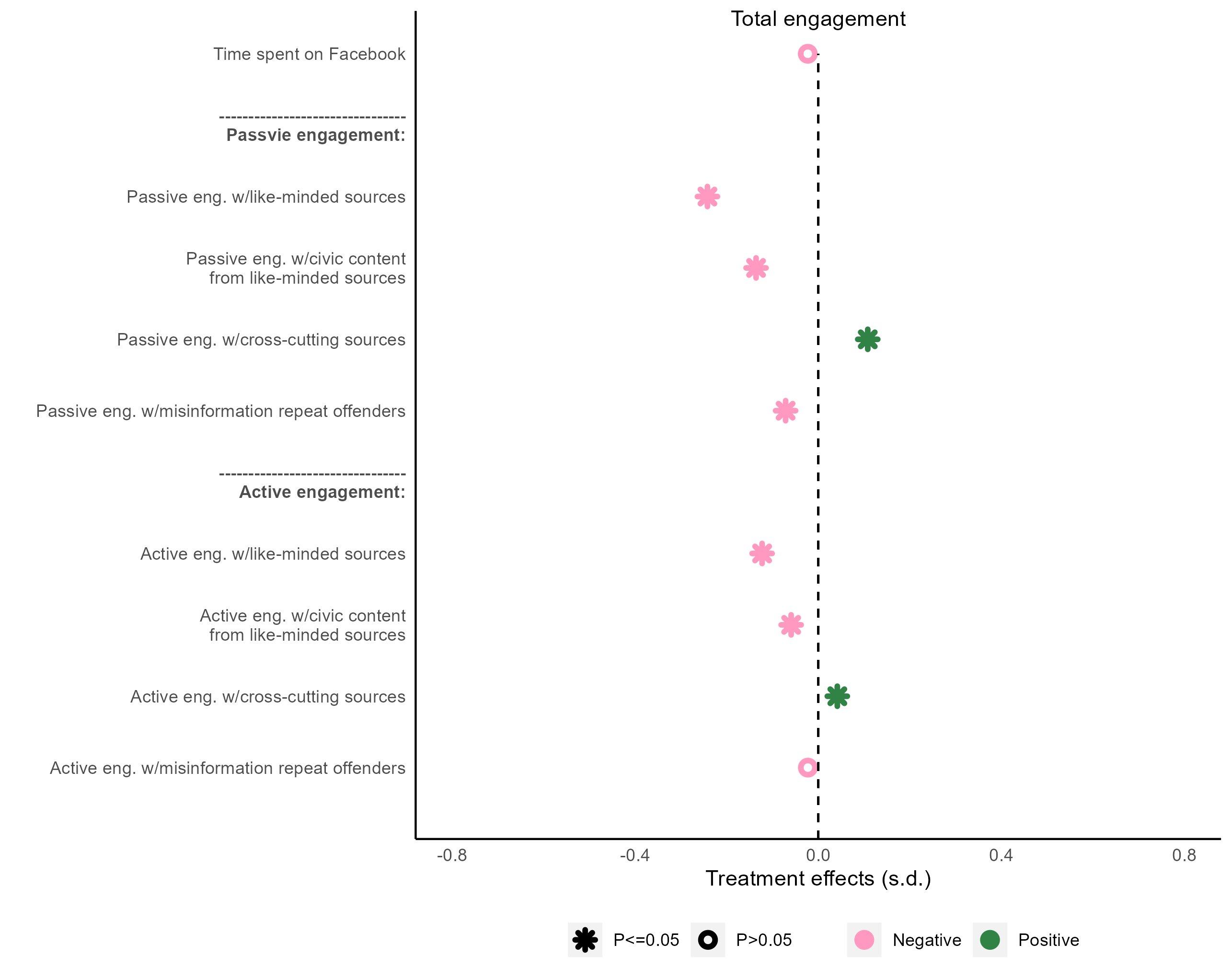
但有一点小trick,就是我们的大类取值是NA,legend会有三类
- Negative
- Poistive
- NA
所以在设置color和shape 时,我们可以用limits这个参数选择,只定义两个level的取值,就可以隐藏到NA这个factor的输出。Nice
fb_figure3_b %>%
  ggplot(aes(x = ate, y = dv_label)) +
  geom_point(aes(color = neg_pos, shape = sig), size = 2, stroke = 2) +
  geom_segment(
    aes(
      x = 0,
      xend = 0,
      y = 0,
      yend = 11
    ),
    color = "black",
    linetype = "dashed"
  ) +
  annotate(
    geom = "text",
    x = 0,
    y = 11.5,
    label = "Total engagement"
  ) +
  # scale_colour_discrete(na.translate = F)+

  scale_color_manual(
    name = "",
    values = c("#FF99BF", "#308344"),
    breaks = c("Negative", "Positive")
  ) +
  scale_shape_manual(
    name = "",
    values = c(8, 1),
    breaks = c("P<=0.05", "P>0.05")
  ) +
  scale_y_discrete(
    name = "",
    limits = rev(levels(fb_figure3_b$dv_label))
  ) +
  scale_x_continuous(
    name = "Treatment effects (s.d.)",
    limits = c(-0.8, 0.8),
    breaks = seq(-0.8, 0.8, 0.4)
  )

  theme(axis.text.y = element_text(face = fb_figure3_b$face)) +
  theme(
    panel.background = element_rect(fill = "white"),
    axis.line = element_line(color = "black"),
    axis.ticks = element_blank(),
    legend.position = "bottom"
  )
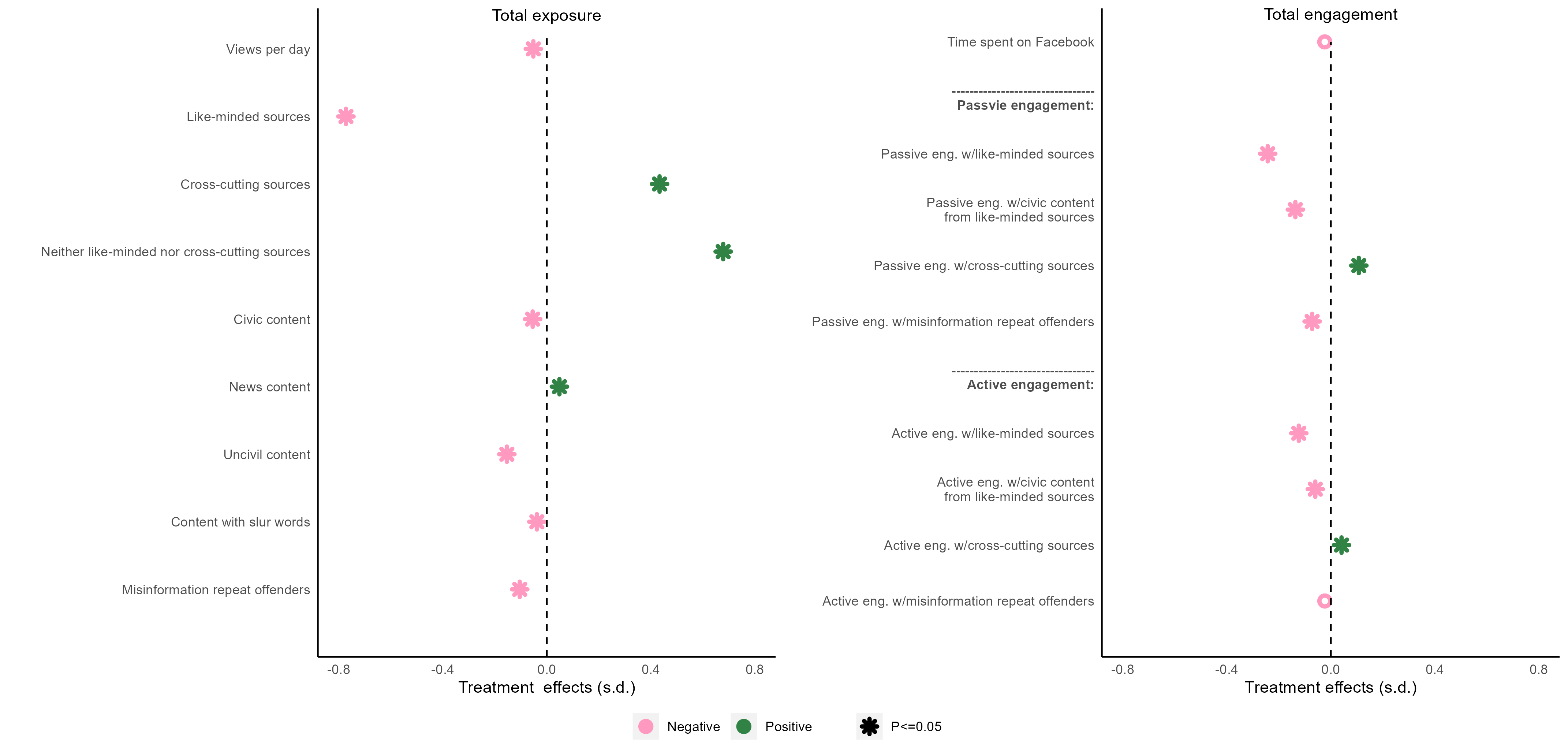
AB 图拼接 🔗
哈哈,最后我们把AB图拼接起来,我首先想到的是ggarrange。有个common.legend = T的选项,可以用第一张图的legend作为合并图之后的legend。但in my case, 我需要用到第二个图的legend,因为第一个图的legend的P-value significance只有一个level(P<=0.05),而common.legend只能取第一个图的legend info。
library(ggpubr)
ggarrange(f3_a, f3_b,
  common.legend = T,
  align = c("hv"), legend = "bottom"
)
ggarrange输出如下:
转而先用get_legend()函数获取想要的legend,然后把ta和我们的AB图用grid.arrange拼装起立就行
- get_legend()之后可以用as_ggplot()把对象用图形形式显示出来
- grid.arrange(),人如其名,非常灵活,可以定义不同的网格拼图。每一个小单元可以用arrangeGrob组合起来,然后再和其他的图形进行拼接。
shared_legend <- get_legend(f3_b)
## as_ggplot(shared_legend) 查看legend
grid.arrange(
 arrangeGrob(f3_a + theme(legend.position = "none"),
   f3_b + theme(legend.position = "none"),
   ncol = 2
 ),
 shared_legend,
 nrow = 2, heights = c(10, 1)
)
最后的效果图如下:
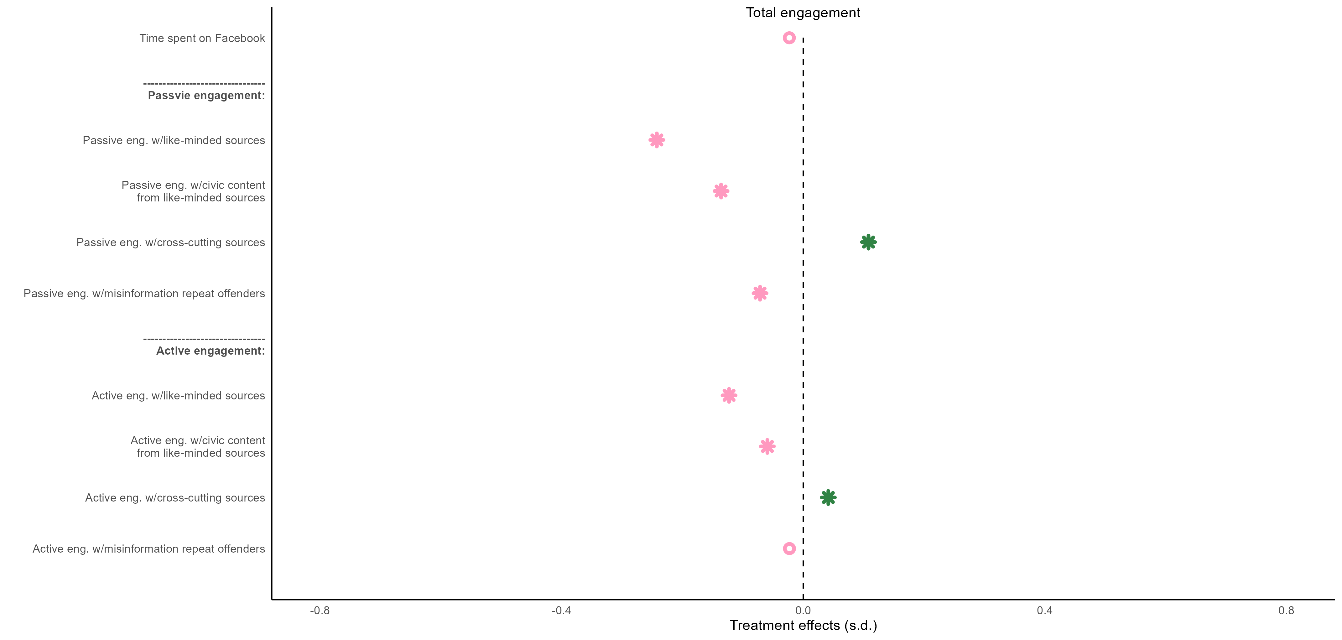
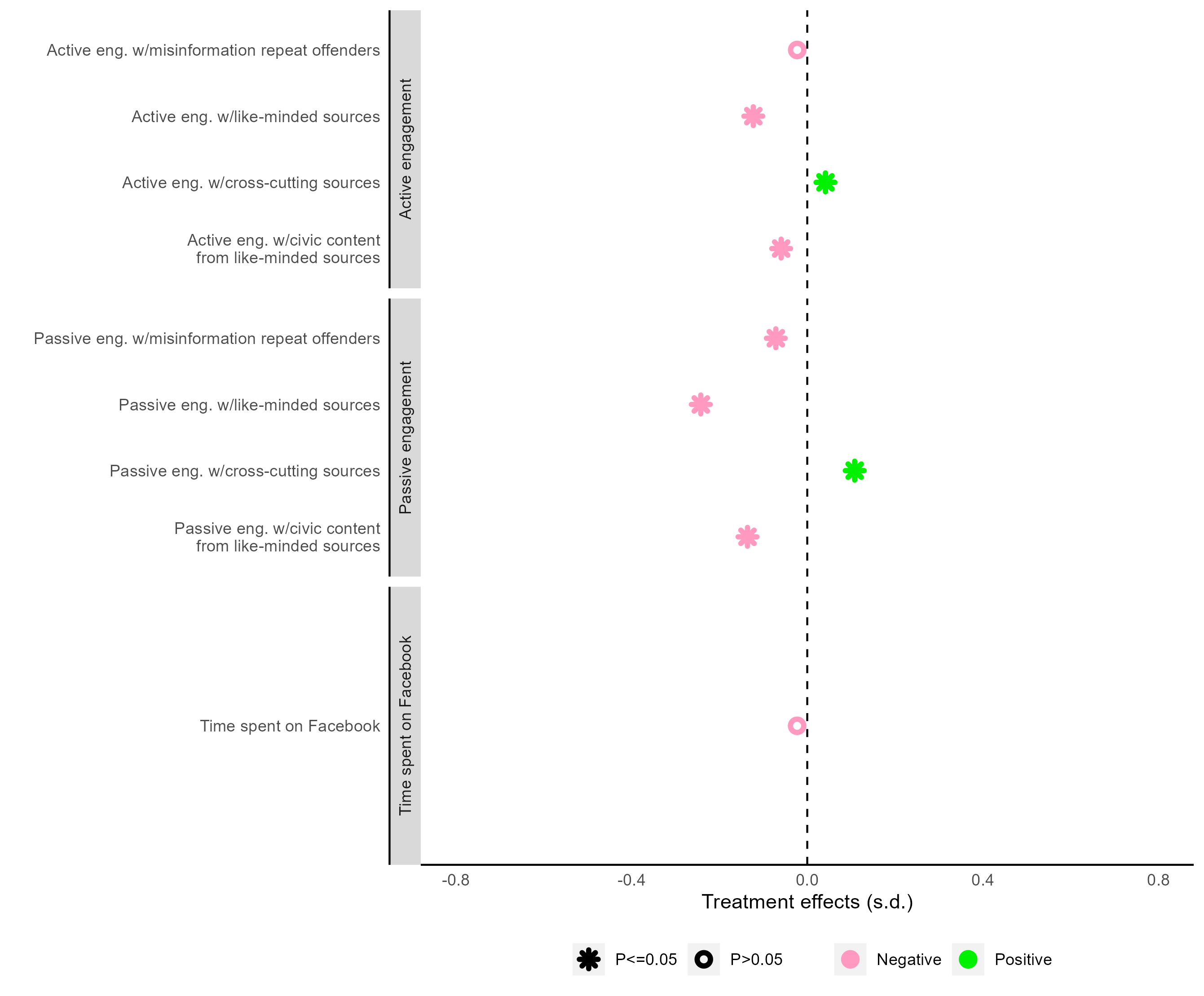
后记:同事建议B图中的横线(我画的虚线)可以用annotate方式加上去? 后后记:对于B图,我们也可以用facet来画,和原图有些许不一样
先生成一个cat变量,这个是大类:
fb_figure3_b2 <- fb_figure3 %>%
  filter(str_detect(facet_label, "B\\)")) %>%
  mutate(
    neg_pos = ifelse(ate < 0, "Negative", "Positive"),
    sig = ifelse(pval <= 0.05, "P<=0.05", "P>0.05")
  ) %>%
  mutate(cat = case_when(
    str_detect(dv_label, "Passive") ~ "Passive engagement",
    str_detect(dv_label, "Active") ~ "Active engagement",
    TRUE ~ "Time spent on Facebook"
  ))
在之前的基础上,增加facet_wrap函数即可:
fb_figure3_b2 %>%
  ggplot(aes(x = ate, y = dv_label)) +
  geom_point(aes(color = neg_pos, shape = sig), size = 2,stroke=2) +
  geom_vline(xintercept = 0, linetype = "dashed") +
  scale_color_manual(
    name = "",
    values = c("#FF99BF", "#00F100")
  ) +
  scale_shape_manual(
    name = "",
    values = c(8, 1)
  ) +
  scale_y_discrete(name='')+
  theme(
    panel.background = element_rect(fill = "white"),
    axis.line = element_line(color = "black"),
    axis.ticks = element_blank(),
    legend.position = "bottom"
  )+
  scale_x_continuous(
    name = "Treatment effects (s.d.)",
    limits = c(-0.8, 0.8),
    breaks = seq(-0.8, 0.8, 0.4)
  )+
  facet_wrap(~cat,
    ncol = 1, dir = "v",
    strip.position = "left", scales = "free_y"
  )
最后输出结果: